Data Project

UMW 2022-2023 Grade Distribution Summary Report

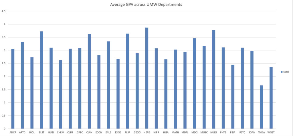
A chart comparing the average GPA of the different departments at the University of Mary Washington.
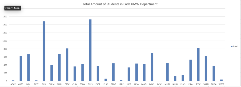
A chart comparing the amount of students in each of the departments at the University of Mary Washington.

The Trends

I chose to focus specifically on the average of the GPA’s of each department at UMW. I found that the departments such as HEPE, NURS, and BLST had the highest average GPA, while departments such as THDA, PSIA, and WGST having the lowest average GPA. The most prominent trend that I could identify was that the departments with the least amount of students would have the highest grade point averages. This could be due to how the average of the the departments with the lowest amount of students are calculated differently to those with a higher amount of students. Another trend is that the departments that are more science-based have a lower average gpa possibly due to the intense curriculum.

The Process

I can admit I do not have a lot of experience at all with spreadsheets. I found any videos, specifically Professor Berge’s video on how to use Microsoft Excel, very helpful, as they explained thoroughly how to accurately analyze data using Excel. I used Microsoft Excel in order to create the data sheet. It made it easy in order to clean up any data that I did not need or anything that wouldn’t be relevant to the trend that I identified. I found the data that I used on the UMW’s site for Institutional Analysis and Effectiveness. They have all the grade distribution summaries dating back to 2017, even including the years during COVID. I specifically used the 2022-2023 Grade Report, as I thought it would be interesting to analyze since those were the years that COVID cases were lowering, and things could go back to normal.

Data Project Checkpoint

Excel Sheet

Here is the link to my excel sheet, and I got my data from Data.gov

Picture of Chart

Chart that shows the average ranking of baby names based on sex and ethnicity.

Identification of Trend

The data records the names and ethnicities of babies that were born in 2011 in New York City, the chart then shows the amount of babies with this name and where its popularity ranking. The trend that I noticed in this graph is that the girls’ names tended to have higher popularity rankings than the boys’ names, no matter the ethnicity.

Methods

To make this graph. I used excel to import my data. The original chart originally had about 69,000 names but I narrowed it down to 1,934 by using only babies who were born in 2011, and by cutting out repeat names and names that were misplaced in the wrong grouping. For example, the ethnicity and genders of the baby names tended to be grouped together, but throughout the chart there would be random white female names in the wrong group. Once I cleaned up the chart, I made a pivot table which was how I noticed that the girl names rank higher in popularity than the boys’. After that, I made a bar graph based on the pivot table.

School Attendance Rates

Checkpoint

While looking through reference linked through previous post to see what type of data I am interested in. I settled on using Conniticuit school attendance rates because I recognized a trend and thought of a possible scenario.

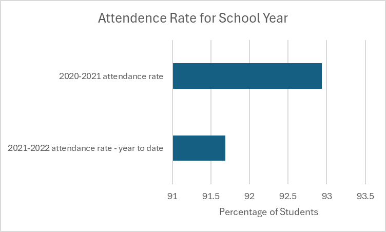
Graph of attendance rate for students in 2020-2021 and 2021-2022.

Trends?

While looking at this graph you can see a large difference between the 2 school years. It is important to look at the percentages because the numbers are not far apart. There is a little over 1% decrease between 20-21 school year to the 21-22 school year. I looked at other variables documented in the data set from Data.Gov. I identified a couple possible reasons on why the attendance rate went down. There is an increase in students with disabilities and students that are homeless in 21-22 school year. This could be a possible explanation to why the attendance rate drops. I used excel to complete everything attached below.

Excel

I pulled all the data into an excel sheet once I got it off of Data.gov. I deleted a couple rows that didn’t have any bearing on the results. I cleaned the data and put it into the table. Once we completed that I pulled the percentages I wanted to graph and created that and added the proper axis titles. After this I used 2 different pivot tables to extract the data I wanted to find the answer to the lowering number.

Data Project Checkpoint

Excel

Chart

Where Found

First, I went to Data.gov and then I found a topic about fruit and vegetable prices, and I thought that was interesting. The actual data was downloaded from USDA.

Explain Trend

The price per pound of fruit rises as the size of the fruit gets smaller.

Process

I just looked at the pivot table and the numbers in excel to determine the trend.

Data Project Checkpoint

Virginia’s Reading Report Card, 4th Grade

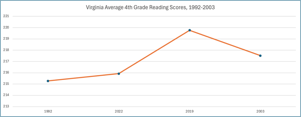
This is a line chart showing that the Virginia reading scores of 4th graders increased from 1992-2019, then decreased from 2019-2003
Chart showing Trend in Virginia Reading Scores. Data from The Nation’s Report Card

Trend

Overall, although the rate of 4th-grade children reading at the basic level was increasing from 1998 to 2019, it has declined from 2019 to 2022. The rate of 4th-grade children reading at the proficient level, which is 238, is significantly lower in 2022 than five years ago.

Process to Identify the Trend

I exported reading score data from The Nation’s Report Card into Excel. The data was collected at four different points in time between 1992 and 2002. It reports on the average score and the reading score percentiles of 4th graders from all 50 states, per collection year. I created a Pivot Table to show the average score per year for only Virginia. For 1992, some states did not collect data so I had to clean up this data before creating the Pivot Table. This is the data that I used to create my chart.

Data Link

The Nation’s Report Card

Spreadsheet and Table Link

The nations report card.xlsx

Data *Test*

Link to data file

This is a link to the data file via Google sheets.

Charts as image

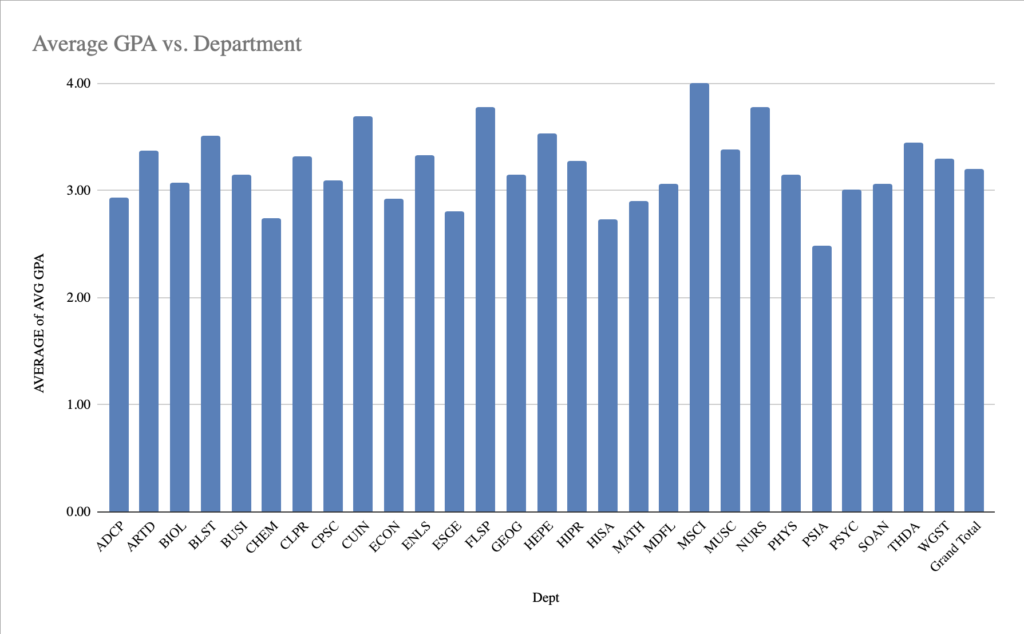
Chart of average GPA vs. department.

This is a chart of the average GPA’s per each department at UMW.

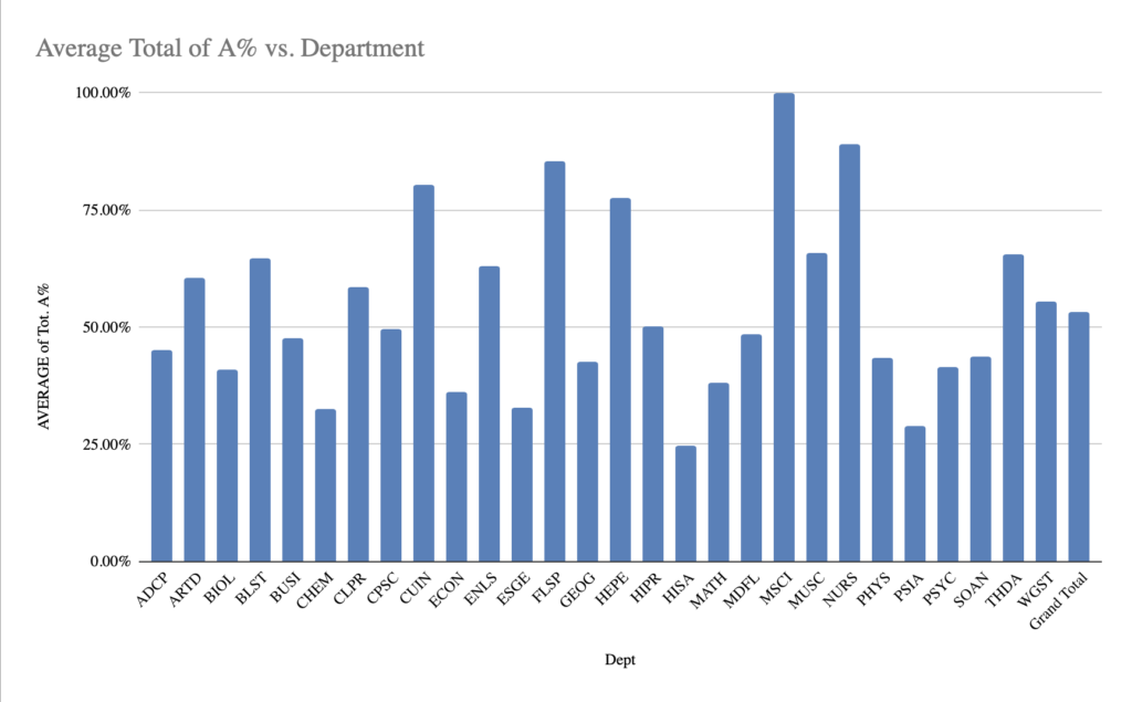
Charr of average total of A% vs. department.

This is a chart of the total of A% compared to each department. This is my trend analysis chart.

Link to dataset source

I found my data source from this website. I chose 2022-2023 grade distribution summary and focused on the undergraduate spring semester of 2023.

Trend explanation

For my trend analysis, I decided to analyze the average percent of A’s in each department. First, I found the average GPA’s in each department, and from there, I found the average percent of A’s. From these charts, I found that the lower the GPA for a class, the lower the A% average. For example, the PSIA department, or Political Science and International Affairs, had only a 2.5 average GPA. And only 26% of the students that semester received an A.

Process explanation

I used Google Sheets to help identify the trend. I put the data into the table and saw the averages for the GPA as well as the A% averages. I wanted to know the correlation between the two so I made separate tables. I was able to put both into pivot charts to easily identify the correlation. A’s in classes significantly help raise a GPA, so that’s why I chose those two different sections of the data.

Special K Chocolatey Delight

My favorite cereal! I had many different favorite cereals over the years: Raisin Bran, Krave, Fruity Pebbles. But in the end of my cereal eating era (there are only two I eat from time to time now), it was the Special K Chocolatey Delight that had me in a chokehold.

Have you walked into cereal aisles recently? There are like, a thousand options. That’s a lot of nutrition labels to read…

That’s why the data set I chose for this ‘Data Project’ is a cereal dataset!

My Cereal Data

Admittedly, this project was the bane of my existence and my headache the entire week. I don’t use Microsoft often, much less Excel, numbers are not my jam, and I simply didn’t (genuinely) have time to go to the DKC for help (which was part of my headache). I like making pretty things and looking at pretty things. Very different. I don’t like how my charts or tables look but I am so ready to stop looking at them. I digress, nothing is easy when you first do it, so a little struggle is healthy, but respectfully, I am so glad that this part is over:P

I got my cereal data from Kaggle btw!

Trend

So, I know we all had a moment in our upbringing when someone told us that cereal isn’t healthy and it was like this crazy realization so much so that we went into a rabbit hole of cereal nutrition labels (…no? Just me?), so instead of focusing on things like sugar and carbs which we all know cereals tend to have a quite a bit of, I wanted to see if there were any trends between any other parts of the nutrition labels. What I found (and chose to focus on) was that a strong positive correlation exists between fiber and potassium, indicating that cereals high in fiber are also likely to be high in potassium and cereals manufactured by Nabisco tend to have the highest average fiber content (therefore, they also have a higher average potassium content per serving)! Yay for no muscle cramps and regularity, if you know what I mean…

How?

How did I find this trend? Well, after I loaded the downloaded and loaded the data into Excel, I went through and deleted and columns and rows that I didn’t find relevant or didn’t want to analyze. I made a chart using the ‘Format as Chart’ button in Excel, and inserted a Pivot Table using that button. With the Pivot Table feature, you can make your own perfect storm of variables that you want to look at next to each other so that its easier to compare and well, analyze. I spent the most time doing this. I clicked around, adding and taking away different nutritional variables but always keeping the cereal name present. In the value field, I made sure I always had ‘average’ instead of ‘sum’ that way I was always looking at the averages of the numbers in front of me instead of what they added up to be. Everything I said is basically everything Professor Berge goes over in this video. Once I thought I saw a trend (the one I mentioned earlier), I asked ChatGPT how to calculate a correlation because I wanted to make sure I wasn’t just imagining it (lol) and these are the instructions it gave me:

  1. Click on an empty cell where you want to display the correlation value.

2. Enter the formula: =CORREL(range_fiber, range_potass), replacing range_fiber and range_potass with the actual cell ranges for the fiber and potassium columns, respectively (e.g., =CORREL(B2:B101, C2:C101)).

3. Press Enter to calculate the correlation. The result will indicate the strength of the relationship between fiber and potassium. A value close to 1 indicates a strong positive correlation.

…To which the value was 0.90! I was not, in fact, imagining it.

That’s when I decided to move some more values around and see which manufacturers cereals tend to have the highest fiber and potassium contents and I landed with Nabisco. I didn’t make a chart for that, however (Remember? Bane of my existence?).

Chart displaying the average fiber and potassium contents of several cereal brands sorted by manufacturer.

So, All-Bran with Extra Fiber does, in fact, beat the rest of cereals in fiber content. Period.

Thank you for coming to my…Blog talk?

Data Point Checkpoint

Data Set and Chart

My Data Set

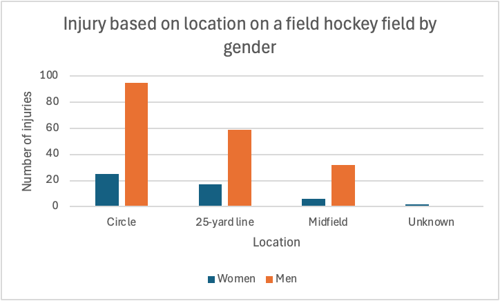
A bar graph that shows the relationship to how many injuries players face in relation to where on the field, displaying men and women

Link to my DataSet

Injury Data of Field Hockey Players

Trend

I noticed that as the players get further from the goal, the injuries decrease. The circle is the place on the field which is closest to the goal, which appears to have the most injuries with men and women. The mid field is the farthest location from the goal, as it appears that is where the least amount of injuries occur.

My Process

After finding the dataset, I copied it into excel. Then, I cleaned up the data, making it look better and more organized. After that, I created the Pivot Table, which displayed the data in a more clear way. Finally, I made a bar graph to visually show the data. These methods helped me determine the trends of the dataset.

Data Project Checkpoint

Spreadsheet

Chart

Screenshot of chart depicting tobacco use depending on race.

Overall Dataset

National Adult Tobacco Survey

Trend

The overall trend that is visible in this data set is that cigarette use is the most common form of tobacco use across all races. Also, it is evident that all forms of tobacco use are most common among white people.

Process

The process I used was pretty simple. I first downloaded the data set from data.gov as an Excel file. I then cleaned my data by removing empty datapoints and irrelevant information to the point I was trying to prove. I had some previous experience using Excel, so I didn’t struggle with the overall cleaning process, but watched the informational video from Canva to show exactly what should be kept/ removed. Trying to figure out the point I wanted to make was probably the most time consuming part of this project. The overall NATS shows race, education level, gender, etc. along with tobacco use, so there were many options for what I could’ve chosen. After finally deciding my point, I then went through each chart to decide which showed this relationship the clearest.

Data Trends in Obesity

Bar graph displaying the rate of obesity from highest percentage to lowest percentage.

Data as a storyteller

Multiple mediums can be used to tell a story, such as film or text. However, numbers can provide a quantifiable story in their own right. Datasets can be used to identify trends that emerge in various topics, that a more qualitative method if inquiry could ignore. One such case is that of the rate of obesity in the United States. While obesity is a national problem and the rate is ever increasing, one region in particular seems to be hit exceptionally hard by this health problem. The data shows that southern states rank especially high in regards to their obesity rate. In fact, nine out of the top ten most obese states are located in the southern United States. The only exception is Kansas, which is firmly outside the southern United States according to the geography of Britannica. From looking at the data the other regions of the United States seem to be more varied in their obesity rates depending on the individual state. No other single region is as heavily represented as the Deep South. This implies that there is something within the socioeconomic or cultural factors in the southern states that leads to a higher rate of obesity than in other regions of the country.

Methodology

The data on obesity rates intrigued me as exercising and fitness are hobbies of mine, and I was able to source the relevant data from the local government of Lake County, Illinois via Data.GOV. I used Microsoft Excel in order to build the data out into a pivot chart, fortunately the data was looking at the obesity rate from a state level and there was not a lot that needed to be cleaned up for the purposes of this examination. I sorted the data by the sum of obesity in a descending order. I then noticed that many of the highest rates were in the southern United States. The chart posted above, helps to show the severity of the Deep South’s obesity rate by illustrating the rate being well over 30% in some of those states. Excel made it easy to load a dataset into a table and then turn said table into a chart.

Excel Spreadsheet:

css.php