Data-Driven Storytelling

Media Project

Adult Depression Rate Infographic

Data

Clean Data Set

Original Data Set

The Story

Overall, the data shows that depression rate is pretty consistent across races. On average, individuals of ‘other’ ethnicities and races have higher rates of depression. White individuals have on average, the second highest depression rates, followed by black, hispanic, and then asian/ pacific islanders. Another interesting find is that there was, on average, a slight increase in depression rates across all races in 2017. Oppositely 2012 had the lowest average depression rates across all races. As a psychology major, it is not uncommon to learn about the unequal availability of treatment. I feel that maybe the discrepancy between races could potentially be attributed to that. Because white individuals are of the majority, they have more access and better treatment than those of a minority group, thus possibly accounting for the much higher diagnoses.

Why I chose this Media & How it Supports the Story in the Data

I chose this infographic because I like that it allows you to see how the races stack up together within the same year. I find the discrepancy between races so interesting and I feel that this infographic allows my readers to interact with each data point individually. In doing so, they are more able to get a sense of how depression rates stay consistent per race over time, but how the individual races vary. I think that being able to see each year in its own section, really shows how big of a difference there is in diagnoses of depression across race.

Process

I honestly really struggled creating this media. Getting a hang of Storyline was the most difficult. Figuring out how exactly my data would be presented and what I wanted shown were the first step in the process. Once I figured that out, I played around with Storyline to show my data in the best way possible. The worst part of the process was getting it embedded to this post. For some reason, I struggled tremendously and could not get it to embed, which I think is because Storyline is not an accepted platform for embedding on WordPress.

Credits & Attribution

Data retrieved from Data.gov, adult depression (LGHC indicator) dataset. Published by California Department of Public Health. https://catalog.data.gov/dataset/adult-depression-lghc-indicator-627e3.

Graphic created by Alexa Kincaid via Storyline.

Obesity Rate of States

Powered By EmbedPress

Story of a dataset

Obviously obesity is a major health risk and is increasingly a talking point in the medical and public health fields. However, visually displaying the data can make the problem more easily understood. I chose to display the data in a map, where higher rates obesity are represented by darker coloration within the corresponding states borders. When displayed like this on a map of the United States, it jumps out to viewers that the Southern United States is far more obese than other regions. Particularly, the Gulf states of Alabama, Mississippi, and Louisiana are the most obese in the nation. The data was compiled by Lake County, Illinois but was found on Data.gov. The information primer on obesity was courtesy of the World Health Organization.

How I did it?

I chose to create a map, with higher rates of obesity being colored darker on the map. I feel that this represents the story I was trying to tell, which was that Southern states have a higher rate of obesity, better than a simple bar graph. Although, I did include the bar graph, which was made with Microsoft Excel, within the PowerPoint presentation to give viewers further numerical information. The map of the US was made via Flourish, a data visualization software. I wanted to make a short PowerPoint presentation because it would convey a short primer of what obesity is, with a short analysis of the map and bar graph. I chose to use PowerPoint because I am familiar with the software and it allowed me to create a simple presentation to convey the story using the data I found. I ran into a challenge embedding a PowerPoint presentation, but managed to get into embedded by downloading a plugin EmbedPress, which allowed me to upload a document to my blog post.

Attributions

Information on Obesity from World Health Organization.

Dataset regarding obesity: data.gov

Software used: Flourish

Image in PowerPoint from freepik.com

Data Project Checkpoint

UMW Institutuinal Analysis & Effectiveness: Grade Distributuion Report: 2023-2024 Grade Distribution Summary

Grade Distribution Report 2023-2024

Undergrad Students per Department

Letter Grades per Department

What I found

While looking through the grades that were earned for the Spring semester of 2024 and the number of students that are enrolled in the different departments I noticed that Business has the largest enrollment of students. However, they do not have the hightest average grade point average. What also needs to be evaluated though is the fact that the CLPR department has a substancially lower nubmer of students than the Business Department. This causes the data to be greatly different and possibly ineffective.

Data Project 9.6 Check Point

Selection of Data Set

I got the data of education, unemployment, poverty and population from data.org. I downloaded the data in an excel format. The data covers all the States including Puerto Rico. The data for education, unemployment and population have time series.

Cleaning the Data

I wanted to focus on Virginia so I deleted the data for the States that are not needed. I also deleted other columns such that have values and not rates. This is because due to difference in for example size, economic activities, etc., I wanted to focus on rates which may be comparable. I used the Microsoft Excel software to clean the data format the table and to do the pivot table.

Formatting the Data as Table

In order to prepare the data to be used for the pivot table, I have to summarize the time series by finding and using the averages. I used data on average percent of adults with less than high school diploma, average unemployment rate, average household median income as percentage of State median household income and poverty rate for 132 counties and cities in Virginia. I have to take out Clifton Forge City and Bedford City because they do not have values for the variables above with the exception of education.

Pivot Table

I did the pivot table based on the counties and cities data on average percent of adults with less than high school diploma, average unemployment rate, average household median income as percentage of State median household income and poverty rate. I used the pivot table to find the average , minimum value and maximum value for the variable. For education Buchanan County has about 52% of adults with less than high school diploma from the estimated average with data from 1970 to 2022. Falls Church City has a minimum percent (9.5%) of adults with less than high school diploma. Attached is the excel document with the data for the pivot table, and the data for the pivot chart.

Preliminary Findings

Education may have some effect on unemployment, household income and poverty. The pivot table shows that Buchanan County with the percent of adults without high school diploma has an unemployment rate higher than than Virginia unemployment rate, a median household income that is about half of the Virginia average and a poverty rate which is about 10% higher than Virginia average.

Image

This is the image chart trend of the percentage of adults with less than high school diploma in the US, Virginia, Buchanan County and Falls Church City from 1970 to 2022.

Data Project Checkpoint 9.6

My Data Charts

The final data charts for my project checkpoint

You can view these charts in my Excel Worksheet by clicking the link, “DGST101_DataProject”!

Trends I Identified Within The Data

Listing the specific trends displayed within the data charts listed above

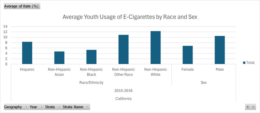
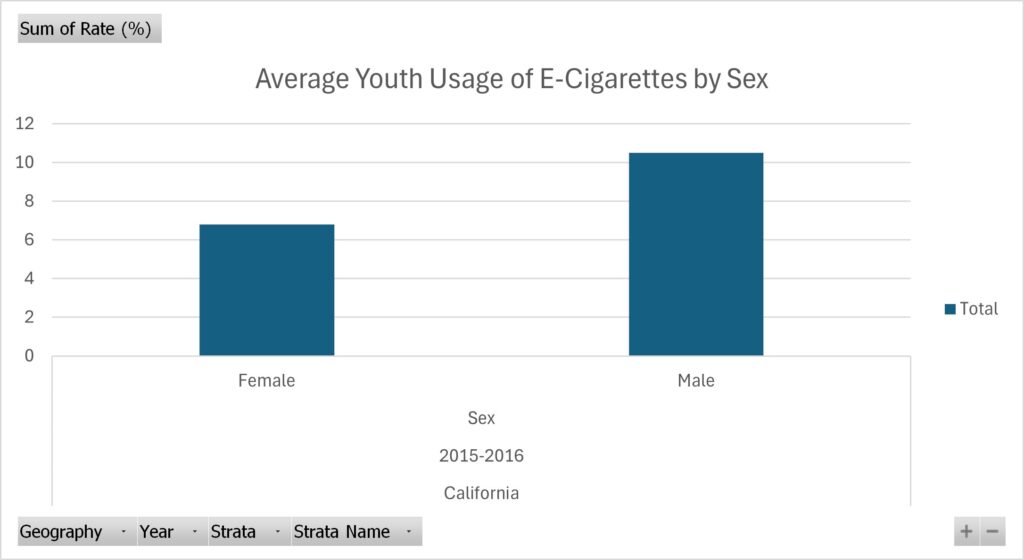
For the data I collected, I chose to inspect trends within the usage of e-cigarettes for the youth. I originally hoped to find some recent research on this done in Virginia. However, I found research done in California instead, and the most recent study I could find was done in 2015/2016. However, I think this is a great state to look at these trends in – since it’s a large state that usually sets many societal trends, including using e-cigarettes. Within the data I collected, I found a trend of white males being the most common perpetrators of e-cigarette usage. I found this data to be extremely interesting, as it defies stereotypes that usually individuals of color are the ones partaking in activities like using e-cigarettes. 

The Process for Finding These Trends

The steps I took to find these specific trends within the data

I found this specific set of data on Data.gov! After a lot of research (and figuring out what story I wish to portray) I found this set of data that really pushed the story I wanted to convey – being that the use of what seems like deviant acts (such as using e-cigarettes) isn’t only by individuals of color, thus another reason why we need to steer clear from this stereotype without doing the proper research. After finding this data, I made use of the cleaning process by watching professor Berge’s video in Canvas. I removed the column that displayed the grand total of individuals that partook in the study, as well as the lower and upper 95% confidence interval because it was irrelevant information to the point I was trying to make. Therefore, once I finished cleaning the data, I isolated the different trends I wanted to highlight in their own pivot tables: one for the sex and the other for the ethnicity of youth that partakes in using e-cigarettes. I did all of this using Microsoft Excel. 

Examining Education Majors at UMW- Data Project Check In

Topic and Trend

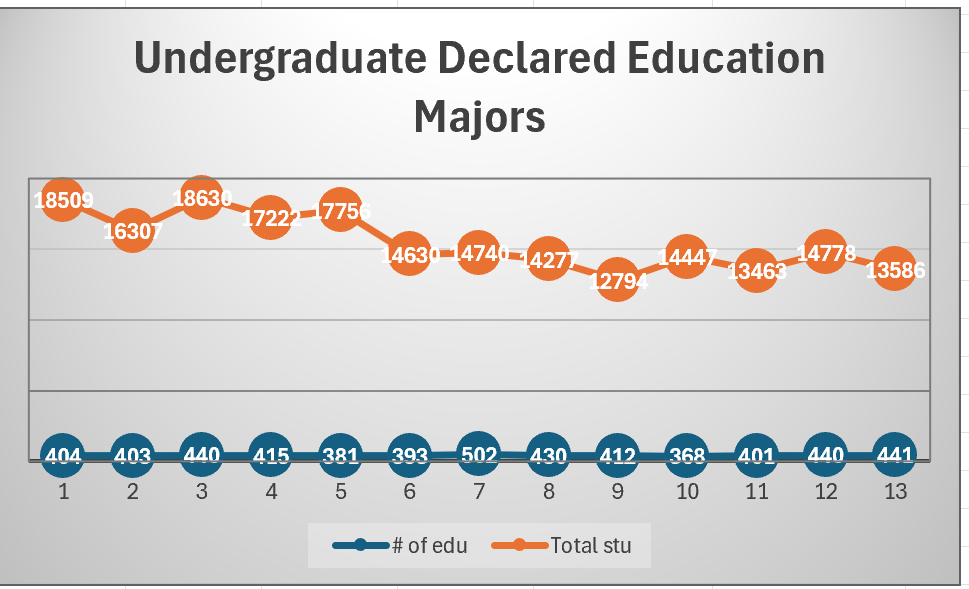
For the data trend project, I decided to examine the number of declared education majors at UMW compared to the whole student body. The United States is going through a teachers crisis, and I was hoping that examining the number of students majoring in education might explain a trend that mirrors the number of current teachers in the US to try to identify what is causing the shortage in teachers in America today. Examining the data through the table and chart revealed that while the number of students at UMW studying education remained relatively low, the number of education majors remained steady even increased after COVID, though decreased in the the most recent years. I found this data set through the UMW Grade Distribution Report. The full data set can be found through this Excel Sheet.

A chart titled "Undergraduate Declared Education Majors" depicts a first data set, the total number of undergraduate declared students, steadily decreasing over time. The second data set, the number of declared education undergraduate students, steadily decreases and then increases overtime.

Process

The trend of the number of declared education majors at UMW decreasing and then steadily increasing overtime was found through Excel. After looking at the Grade Distribution Report, I copied the number of total declared education majors for each semester onto an Excel sheet (excluding Spring 2020, which did not have any data due to the change in grading systems as a result of the COVID outbreak. After creating a table, I copied the data into a pivot table, which helped me create a more visual line graph to represent the changes in the number of declared education majors and total undergraduate students with declared majors. Through the chart, I was able to identify that the data first decreased, increased, and then decreased overtime. The steady decrease in the years after COVID may represent a possible trend in teaching conditions after COVID, though the data resembled pre-COVID data closely.

Data Project

UMW 2022-2023 Grade Distribution Summary Report

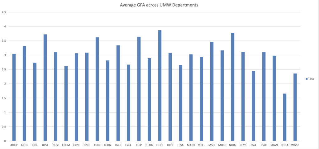
A chart comparing the average GPA of the different departments at the University of Mary Washington.
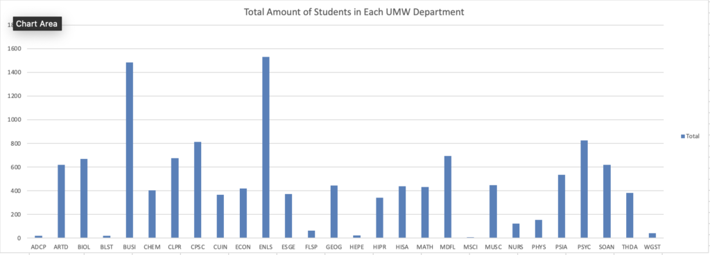
A chart comparing the amount of students in each of the departments at the University of Mary Washington.

The Trends

I chose to focus specifically on the average of the GPA’s of each department at UMW. I found that the departments such as HEPE, NURS, and BLST had the highest average GPA, while departments such as THDA, PSIA, and WGST having the lowest average GPA. The most prominent trend that I could identify was that the departments with the least amount of students would have the highest grade point averages. This could be due to how the average of the the departments with the lowest amount of students are calculated differently to those with a higher amount of students. Another trend is that the departments that are more science-based have a lower average gpa possibly due to the intense curriculum.

The Process

I can admit I do not have a lot of experience at all with spreadsheets. I found any videos, specifically Professor Berge’s video on how to use Microsoft Excel, very helpful, as they explained thoroughly how to accurately analyze data using Excel. I used Microsoft Excel in order to create the data sheet. It made it easy in order to clean up any data that I did not need or anything that wouldn’t be relevant to the trend that I identified. I found the data that I used on the UMW’s site for Institutional Analysis and Effectiveness. They have all the grade distribution summaries dating back to 2017, even including the years during COVID. I specifically used the 2022-2023 Grade Report, as I thought it would be interesting to analyze since those were the years that COVID cases were lowering, and things could go back to normal.

Data Project Checkpoint

Excel Sheet

Here is the link to my excel sheet, and I got my data from Data.gov

Picture of Chart

Chart that shows the average ranking of baby names based on sex and ethnicity.

Identification of Trend

The data records the names and ethnicities of babies that were born in 2011 in New York City, the chart then shows the amount of babies with this name and where its popularity ranking. The trend that I noticed in this graph is that the girls’ names tended to have higher popularity rankings than the boys’ names, no matter the ethnicity.

Methods

To make this graph. I used excel to import my data. The original chart originally had about 69,000 names but I narrowed it down to 1,934 by using only babies who were born in 2011, and by cutting out repeat names and names that were misplaced in the wrong grouping. For example, the ethnicity and genders of the baby names tended to be grouped together, but throughout the chart there would be random white female names in the wrong group. Once I cleaned up the chart, I made a pivot table which was how I noticed that the girl names rank higher in popularity than the boys’. After that, I made a bar graph based on the pivot table.

School Attendance Rates

Checkpoint

While looking through reference linked through previous post to see what type of data I am interested in. I settled on using Conniticuit school attendance rates because I recognized a trend and thought of a possible scenario.

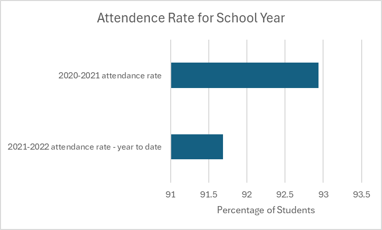
Graph of attendance rate for students in 2020-2021 and 2021-2022.

Trends?

While looking at this graph you can see a large difference between the 2 school years. It is important to look at the percentages because the numbers are not far apart. There is a little over 1% decrease between 20-21 school year to the 21-22 school year. I looked at other variables documented in the data set from Data.Gov. I identified a couple possible reasons on why the attendance rate went down. There is an increase in students with disabilities and students that are homeless in 21-22 school year. This could be a possible explanation to why the attendance rate drops. I used excel to complete everything attached below.

Excel

I pulled all the data into an excel sheet once I got it off of Data.gov. I deleted a couple rows that didn’t have any bearing on the results. I cleaned the data and put it into the table. Once we completed that I pulled the percentages I wanted to graph and created that and added the proper axis titles. After this I used 2 different pivot tables to extract the data I wanted to find the answer to the lowering number.

Data Project Checkpoint

Excel

Chart

Where Found

First, I went to Data.gov and then I found a topic about fruit and vegetable prices, and I thought that was interesting. The actual data was downloaded from USDA.

Explain Trend

The price per pound of fruit rises as the size of the fruit gets smaller.

Process

I just looked at the pivot table and the numbers in excel to determine the trend.

css.php